A/B Testing
A/B Testing
Imagine that you’ve got a great product and a beautiful website with plenty of visitors, but and here’s the rub … not as many sales as you’d like.
There are all kinds of changes you could make, but the important thing is how can you tell whether whatever it is that you’ve changed has made a difference? And how can you tell whether or not any differences are down to chance?
It turns out that there’s a tried and tested way of finding these things out and thats called A/B Testing.
To run A/B tests you create two different versions of something - usually versions of a webpage, and then randomly serve 1 of them to a user, creating a simple randomized trial. You then record whether the user converts to making a sale or perhaps creating an account or whatever it is you wish to achieve.
A/B testing lets you compare version A - usually your current or control option, with version B the new option. Then you are able to compare the convertion rates of A and B and see whether there are any differences and whether those differences are significant.
We’ll begin our project by simulating some data with different convertion rates using different binomial distributions.require(dplyr)
require(ggplot2)
require(cowplot)
# decide how many samples
size <- 1000
# create 4 different page simulations
# with different convertion rates
pages <- data.frame(group = c('Control', 'A', 'B', 'C'),
c.rate = c(0.03, 0.05, 0.02, 0.08),
stringsAsFactors = FALSE)
# seed for reproducibility
set.seed(1234)
control <- rbinom(size, 1, pages$c.rate[1])
a <- rbinom(size, 1, pages$c.rate[2])
b <- rbinom(size, 1, pages$c.rate[3])
c <- rbinom(size, 1, pages$c.rate[4])
# put into a (tidy) dataframe
df <- data.frame(page=rep(x = c('Control', 'A', 'B', 'C'), each=size),
converted=c(control, a, b, c),
stringsAsFactors = FALSE )
Looking at some summary statistics for our simulated data:# get some summary stats
df %>%
group_by(page) %>%
summarise(Num=n(),
num.converted=sum(converted),
num.n.converted=n()-sum(converted),
c.rate.sim=100*mean(converted)) %>%
left_join(pages, by=c("page" = "group")) %>%
mutate(c.rate=100*c.rate)## # A tibble: 4 x 6
## page Num num.converted num.n.converted c.rate.sim c.rate
## <chr> <int> <int> <int> <dbl> <dbl>
## 1 A 1000 33 967 3.3 5
## 2 B 1000 21 979 2.1 2
## 3 C 1000 86 914 8.6 8
## 4 Control 1000 42 958 4.2 3
To assess whether our two pages convertion rates are actually different we need to perform a hypothesis test. Our null hypothesis, H0, is that our 2 pages convertion rates are equal, whereas our alternate hypothesis, HA, is that they differ.
Pearson’s chi-squared test of independence
If our samples are large enough and our convertion rates aren’t near 0 or 1, then we can use Pearson’s chi squared test.
This will give us a p value, which tells us the probability of getting results this extreme (or more) - assuming that the null hypothesis is true. So if our p-values are small (p < 0.05 is usual) then we can assume that the null hypothesis is unlikely enough, so we can accept the alternative hypothesis.
Comparing our Control with A, B & C
Comparing Control and Adf %>%
filter(page=='Control' | page=='A') %>%
group_by(page) %>%
summarise(num.converted=sum(converted),
num.n.converted=n()-sum(converted)) %>%
select(-page) %>%
chisq.test()##
## Pearson's Chi-squared test with Yates' continuity correction
##
## data: .
## X-squared = 0.88658, df = 1, p-value = 0.3464
Comparing Control and Bdf %>%
filter(page=='Control' | page=='B') %>%
group_by(page) %>%
summarise(num.converted=sum(converted),
num.n.converted=n()-sum(converted)) %>%
select(-page) %>%
chisq.test()##
## Pearson's Chi-squared test with Yates' continuity correction
##
## data: .
## X-squared = 6.5557, df = 1, p-value = 0.01045
Comparing Control and Cdf %>%
filter(page=='Control' | page=='C') %>%
group_by(page) %>%
summarise(num.converted=sum(converted),
num.n.converted=n()-sum(converted)) %>%
select(-page) %>%
chisq.test()##
## Pearson's Chi-squared test with Yates' continuity correction
##
## data: .
## X-squared = 15.433, df = 1, p-value = 8.548e-05
Comparing the new pages to our control we get:
| page | p-value | Significant | Convertion Rate | Actual Rate |
|---|---|---|---|---|
| Control | – | – | 3.1 | 3 |
| A | 0.3464 | No | 4.7 | 5 |
| B | 0.01045 | Yes | 1.3 | 2 |
| C | 8.548e-05 | Yes | 8.1 | 8 |
This shows that page A isn’t significantly different to the control, any difference could be down to chance.
Page B is significantly different to the control, however the convertion rate is lower than the control.
Page C is significantly different to the control, and the convertion rate much higher. This would be the page to change to.
Visual Comparison
If we create a monte carlo simulation of our web hits and convertions then we can get a visual comparison to check whether our results make sense.# get sample distributions
each.sample.size <- 250
num.samples <- 100
getMean <- function(nIndex, num) {
mean(sample_n(df %>% filter(page==pages$group[nIndex]), num)$converted)
}
s.con <- data.frame(page=pages$group[1],
c.rate=replicate(num.samples, getMean(1, each.sample.size)))
s.a <- data.frame(page=pages$group[2],
c.rate=replicate(num.samples, getMean(2, each.sample.size)))
s.b <- data.frame(page=pages$group[3],
c.rate=replicate(num.samples, getMean(3, each.sample.size)))
s.c <- data.frame(page=pages$group[4],
c.rate=replicate(num.samples, getMean(4, each.sample.size)))
# combine the sample distributions
s.df <- rbind(s.con, s.a, s.b, s.c)
# get the summary stats
s.df %>%
group_by(page) %>%
summarise(Num=n(),
median=median(c.rate),
sd=sd(c.rate),
min=min(c.rate),
min.05=mean(c.rate)-(1.96*sd),
mean=mean(c.rate),
max.05=mean(c.rate)+(1.96*sd),
max=max(c.rate)
) %>%
left_join(pages, by=c("page" = "group"))## Warning in left_join_impl(x, y, by$x, by$y, suffix$x, suffix$y): joining
## character vector and factor, coercing into character vector## # A tibble: 4 x 10
## page Num median sd min min.05 mean max.05
## <chr> <int> <dbl> <dbl> <dbl> <dbl> <dbl> <dbl>
## 1 Control 100 0.040 0.009609003 0.020 0.022646355 0.04148 0.06031364
## 2 A 100 0.036 0.010187415 0.012 0.014912666 0.03488 0.05484733
## 3 B 100 0.020 0.007504988 0.004 0.007010223 0.02172 0.03642978
## 4 C 100 0.086 0.014375906 0.048 0.058423225 0.08660 0.11477678
## # ... with 2 more variables: max <dbl>, c.rate <dbl># grah the sample distributions for each 'page'
plot.density <-
s.df %>%
ggplot(aes(x=c.rate, colour=page)) +
geom_density() +
theme(axis.text.y=element_blank()) +
ggtitle("Convertion Rate Variance for each Page")
# boxplot using a custom box size
# where the box size is 0.05 < p < 0.95
# and the whisker length is min, max
plot.boxplot <-
s.df %>%
ggplot(aes(x=page, y=c.rate, colour=page)) +
stat_summary(geom = "boxplot",
fun.data = function(x) setNames(quantile(x, c(0.0, 0.05, 0.5, 0.95, 1.00)), c("ymin", "lower", "middle", "upper", "ymax")),
position = "dodge") +
coord_flip() +
theme(axis.text.y=element_blank())
plot_grid(plot.density, plot.boxplot, ncol = 1, nrow = 2)
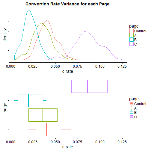
The density plot and box plots both show the same monte carlo generated data to simulate convertion rates.
The boxplot has been modified so that each box size shows 0.05 < p < 0.95 for that page, with the whiskers showing the min/max values, this clearly shows how the distributions overlap.
From these graph it can be seen that:
- Control and A are very similar
- Control and B are similar but significantly different
- Note that the median lines are not within the 0.05 < p < 0.95 range of the other’s box
- Control and C are clearly different
From these visual results it’s also clear that we would choose to use version C of the page.
The github repository for this project can be viewed here.